Introduction
The previous blog examined why fully connected feed-forward networks fail when applied to images. Flattening destroys spatial structure, parameters grow uncontrollably, and the model has no notion of locality or translation.
These limitations made it clear that image recognition required architectural changes, not just better optimization or more data.
Historically, many early neural network ideas were guided by observations from biology—not as literal simulations, but as conceptual constraints. When researchers faced the problem of visual pattern recognition, they again looked toward how vision is processed hierarchically.
This line of thought led to the Neocognitron (1980), proposed by Kunihiko Fukushima—one of the earliest models to explicitly formalize local receptive fields, hierarchical feature extraction, and translation-invariant recognition.
Neocognitron — K. Fukushima (1980)
The Neocognitron is a self-organizing neural network designed for pattern recognition unaffected by shifts in position, directly addressing one of the key weaknesses of traditional feed-forward networks.
Rather than treating an image as a flat vector, the Neocognitron processes it as a spatial structure, enabling progressively more abstract representations to emerge across layers.
Inspired by earlier studies of the visual cortex (notably by Hubel and Wiesel), the model follows a hierarchical progression:
\[\text{simple edges and corners} \rightarrow \text{combinations of features} \rightarrow \text{complete shapes}\]This hierarchy is not hard-coded. Instead, it emerges through a process of self-organization.
Architecture
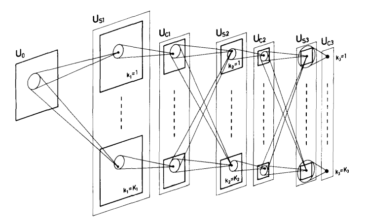
The input layer, denoted as $U_0$, receives the image as a 2D matrix. Importantly, the input is never flattened, preserving spatial relationships from the outset.
The network is composed of repeating modules, each consisting of two types of layers:
S Cells (Feature-Detecting Cells)
S-cells act as local feature detectors. They respond selectively to specific patterns within a limited spatial neighborhood.
We denote the S-layer in the $l$-th module as:
\[U_{S_l}\]Each S-layer consists of multiple S-planes. All cells within a single plane share identical synaptic parameters and therefore detect the same type of feature, but at different spatial locations.
C Cells (Aggregation / Pooling Cells)
C-cells aggregate responses from S-cells and introduce tolerance to small shifts in position.
We denote the C-layer in the $l$-th module as:
\[U_{C_l}\]Each C-plane pools information from a corresponding S-plane over a local region, responding strongly if the feature is present anywhere within that region.
Structural Terminology (Clarified)
To avoid confusion, it helps to distinguish the following:
- Cell: a single computational unit
- Plane: a 2D array of cells detecting the same feature
- Layer: a stack of planes (multiple feature types)
- Module: an S-layer followed by a C-layer
This organization closely anticipates what later became feature maps, convolution layers, and pooling layers in modern CNNs.
Receptive Fields and Depth
As the network progresses deeper:
- receptive fields become larger
- spatial resolution decreases
- representations become more abstract
In the final module, each C-plane contains only one cell, whose receptive field covers the entire input. At this stage, the network responds to complete patterns, regardless of where they appear.
Cell Dynamics and Inhibition
All cells operate on non-negative analog values, representing activation strength rather than binary firing.
Both S-cells and C-cells are excitatory, meaning their outputs increase activity in downstream units. In addition, the model includes inhibitory cells, which regulate responses and enforce competition.
Rather than being biologically interpreted, these inhibitory mechanisms can be viewed functionally as normalization and selectivity controls.
S-Cells in Detail
S-cells receive shunting inhibitory inputs, allowing their responses to be modulated by surrounding activity.
The output of an S-cell in the $k_l$-th plane of the $l$-th module is given by:
\[u_{Sl}(k_l, n) = r_l \cdot \phi\left[ \frac{ 1 + \sum_{k_{l-1} = 1}^{K_{l-1}} \sum_{v \in S_l} a_l(k_{l-1}, v, k_l) \cdot u_{Cl-1}(k_{l-1}, n+v) }{ 1 + \frac{2r_l}{1+r_l}, b_l(k_l) \cdot v_{Cl-1}(n) } - 1 \right]\]where $\phi[x]$ is a ReLU-like nonlinearity.
While the equation may appear complex, its role is straightforward:
- the numerator computes a weighted match between the input and learned feature templates
- the denominator normalizes the response using inhibitory signals
- the parameter $r_l$ controls selectivity
The Role of Selectivity ($r_l$)
The parameter $r_l$ determines how sharply an S-cell responds:
- high $r_l$ → strong selectivity, precise feature detection
- low $r_l$ → broader tolerance to distortions and noise
This introduces an unavoidable trade-off:
- too much selectivity → failure on noisy inputs
- too little selectivity → confusion between similar patterns
Inhibitory Cell $v_{Cl-1}(n)$
The inhibitory cell connected to S-cells computes an RMS-style aggregation:
\[v_{Cl-1}(n) = \sqrt{ \sum_{k_{l-1}=1}^{K_{l-1}} \sum_{v \in S_l} c_{l-1}(v) \cdot u_{Cl-1}^2(k_{l-1}, n+v) }\]This signal provides a measure of local activity strength, allowing the network to evaluate similarity in a normalized manner.
The summation range $S_l$ defines the receptive field for the layer and grows with depth.
How Translation Invariance Emerges
Within a single S-plane, many cells detect the same feature, but at different spatial locations.
When a pattern shifts:
- the originally active S-cell may no longer respond
- another S-cell in the same plane becomes active instead
C-cells then pool over these responses, ensuring that recognition depends on feature presence, not exact position.
This mechanism directly addresses one of the fundamental limitations of MLPs.
C-Cells in Detail
C-cells also receive shunting inhibitory inputs, but their outputs exhibit a saturating characteristic.
The output of a C-cell in the $k_l$-th plane of the $l$-th module is:
\[u_{Cl}(k,n) = \psi\left[ \frac{ 1 + \sum_{v \in D_l} d_l(v), u_{Sl}(k_l, n+v) }{ 1 + v_{Sl}(n) } - 1 \right]\]where
\[\psi[x] = \varphi\left(\frac{x}{\alpha + x}\right)\]Interpretation
Functionally, C-cells behave like soft pooling units:
- nearby S-cell activations contribute more strongly
- distant activations contribute less
- saturation prevents runaway responses
The parameter $\alpha$ controls how quickly saturation occurs:
- low $\alpha$ → faster saturation
- high $\alpha$ → extended linear response
Self-Organization and Learning
Learning in the Neocognitron is unsupervised and occurs whenever a pattern is presented.
From each S-layer, a small set of representative S-cells is selected—at most one per S-plane. Only these representatives and the S-cells in the same plane receive synaptic reinforcement.
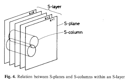
This mechanism ensures that:
- different S-planes specialize in different features
- redundancy is avoided
- feature diversity emerges naturally
Initially, excitatory synapses have small positive values, enabling weak orientation sensitivity. Inhibitory synapses start at zero and grow through learning.
Network Operation After Training
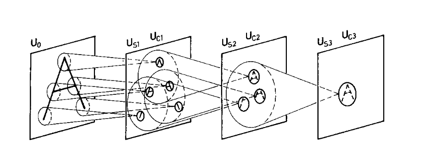
After self-organization:
- early layers detect simple local features
- intermediate layers detect combinations of features
- the final C-layer responds selectively to entire patterns
Each pattern activates one dominant C-cell in the final layer, regardless of its position or minor distortions.
Importantly, many feature planes are shared across patterns, preventing parameter explosion—a key failure mode of MLPs.
Key Takeaway
S-layers ≈ Convolution C-layers ≈ Pooling
The Neocognitron did not use backpropagation, GPUs, or large datasets. What it introduced was more fundamental:
- local receptive fields
- hierarchical feature extraction
- translation-invariant recognition
These ideas formed the structural foundation upon which modern convolutional networks were later built.
Implementation Note
To validate these ideas concretely, the architecture was implemented and trained end-to-end.
The Neocognitron described above has been implemented from scratch in PyTorch, closely following the original formulation by Fukushima, including S-cells, C-cells, inhibitory mechanisms, and unsupervised self-organization.
The implementation, along with experiments and visualizations of learned feature maps and final C-layer activations, is available here:
GitHub: Implementation
TL;DR
The Neocognitron (1980) was an early neural architecture developed to address the failure of fully connected networks on image data. Instead of flattening images, it preserved spatial structure and processed inputs through a hierarchy of locally connected layers. The model is composed of repeating S-layers and C-layers: S-layers act as local feature detectors, with each S-plane detecting the same feature at different spatial locations, while C-layers pool over these responses to introduce tolerance to shifts in position. As depth increases, receptive fields grow, spatial resolution decreases, and representations evolve from simple local features to complete patterns.
Learning in the Neocognitron is unsupervised and self-organizing. For each input pattern, only a small set of representative S-cells are reinforced, forcing different planes to specialize in different features and preventing redundancy. Inhibitory mechanisms regulate activity and control selectivity, balancing robustness to noise against discrimination between similar patterns. Although it predates backpropagation and modern training methods, the Neocognitron introduced the architectural principles—local receptive fields, shared weights across space, hierarchical feature extraction, and pooling-based translation invariance—that later became central to convolutional neural networks.
References
-
Fukushima, K. (1980).
Neocognitron: A Self-Organizing Neural Network Model for a Mechanism of Pattern Recognition Unaffected by Shift in Position.
Biological Cybernetics, 36, 193–202.
https://link.springer.com/article/10.1007/BF00344251 -
Hubel, D. H., & Wiesel, T. N. (1962).
Receptive fields, binocular interaction and functional architecture in the cat’s visual cortex.
The Journal of Physiology.
https://www.ncbi.nlm.nih.gov/pmc/articles/PMC1359523/ -
ScratchMind Blog — Multilayer Perceptron From Scratch — and Why CNNs Were Needed
https://scratchmind.github.io/blog/2025-12-mlp-and-why-cnn/ -
ScratchVision — Neocognitron (PyTorch, from scratch)
https://github.com/ScratchMind/ScratchVision/blob/main/src/models/Neocognitron.py